 Scale-TimeDynamics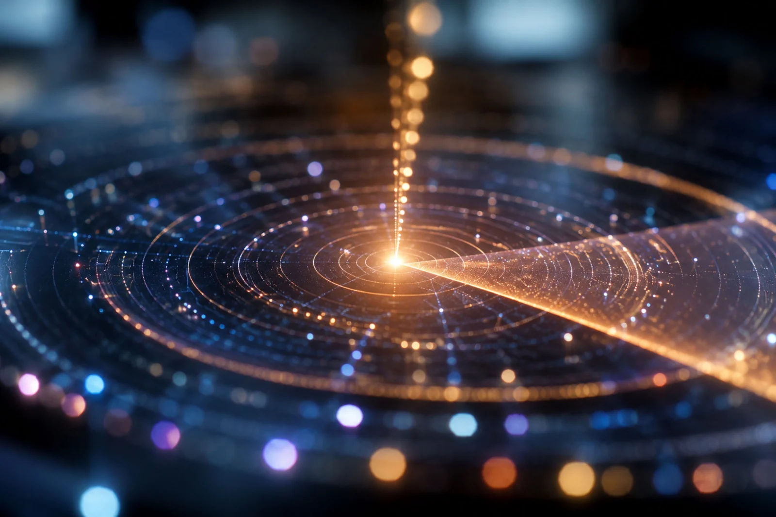
A hundred-year-old crack in physics
Physics has a mystery hiding in plain sight, and it is almost exactly a hundred years old. In the 1920s it became clear that the world of the very small does not behave like the world we live in. An electron does not sit in one place the way a coffee cup does. It carries a spin that cannot be pinned down the way a spinning top can. Measure it one way and you obtain a definite outcome, even though the theory generally assigns probabilities to the possible outcomes beforehand. Quantum theory describes all of this with extraordinary precision. It is the most accurately tested theory in the history of science.
And yet the coffee cup just sits there. Definite place, definite size, definite orientation. It does not flicker and it does not blur.
Here is the crack: both are made of the same stuff. Every stable cup is built out of those flickering quantum parts. Somewhere between the electron and the cup, uncertainty becomes stability. Where exactly, and why?
A great deal of that question already has an answer, and it should be said plainly. Decoherence describes how a system interacting with its surroundings loses the interference between its alternatives, and does so fast enough that nothing as large and as warm as a cup could ever be caught behaving otherwise. It also explains why particular properties, position among them, are the ones that survive to be seen. That work is well established, and nothing in this framework disputes it. What decoherence is widely agreed not to settle on its own is why one definite outcome occurs rather than another, and on that the interpretations still disagree. A century of careful work has produced many partial answers and no single picture that everyone finds satisfying.
Scale-Time Theory proposes that the two are not two kinds of thing at all. They are one relation, read at two different sampling depths.
One sweep, one speed, one step
The framework does not begin with space as a container holding objects. It begins with a rhythm.
Picture a radar screen. At the centre sits a single source, and from it one sweep rotates through everything at an invariant frequency. STT calls this the phasor sweep. It is shared: every relation in the framework is turned by the same beam at the same rate.
Two things travel with it and never change. The carrier speed,
cφ = c, which is the speed of light taken as a primitive of
the framework rather than derived inside it, and which stays the causal ceiling
throughout. And the distance that carrier covers in one turn of the sweep, the
phasor travel step, which calibrates every length in the theory.
The radar image is a teaching device, and the manuscript says so plainly rather than leaving it to be assumed. Scale-space is not claimed to be made of literal rings and clock hands. What the picture buys is a vocabulary: rings are scale horizons, a point on a ring is a phase position, and a line crossing many rings is a baseline, the coupled relation that turns many scale relations into one system.
Scale is path, not size
Put a record on a turntable. The whole disc shares exactly one rotation: the label and the outer rim complete each turn together, same rhythm, same timing. But a point near the centre travels a short groove during that turn, and a point near the rim travels a long one. The rotation is shared; the distance covered depends entirely on how far out you sit.
That is what STT means by scale. A scale relation has a radius, measured in phasor travel steps, and an outer horizon path of two pi times that radius. Sitting at a larger scale is sitting farther out on the record: the same turn of the sweep opens more path for you.
Notice what does not change. The carrier speed is invariant. Scale does not make the rhythm faster or slower. It changes how much distance one turn of the rhythm contains.
The framework also carries an area-like label for a scale relation, its
scale address σ = πR², alongside a dimensionless form
used for sampling. Because the address is area-like while radius and path are
length-like, any ratio mixing the two families carries a square root: double the path
and you quadruple the address. It is a small piece of bookkeeping, and it runs
through the whole document.
From scale address to sampling depth
Now the two halves have to be joined, and this joint is what carries the framework.
A standing pattern living at a given scale address has a cadence of its own. What
matters is not that cadence in isolation but its ratio to the shared sweep: how many
samples of the sweep fall inside one cycle of the pattern. That ratio is written
RA, and the link from address to ratio is the
scale-to-sampling bridge.
Version 11.0 states one property of that link, openly, as its single postulate:
Within a family of standing scale modes, the sampling ratio increases with the scale address. Larger and slower relations sit deeper in resolvable territory; smaller and faster relations sit nearer the sampling edge.
The manuscript is unusually direct about why this is stated rather than shown. Without some stated property of the bridge, the central correspondence between scale and sampling regime has no carrier and cannot be tested at all. Its functional form and its calibration are untested, and the named route to testing it is a nested-ladder simulation in which mode cadence is derived from scale address rather than scanned directly.
It is also the formal carrier of the line this whole project started from: an unresolved edge in the small scales, and completed appearance in the large ones.
The zoetrope, and what a baseline is
A zoetrope is a Victorian toy: a drum with narrow slits cut into its side and a strip of drawings inside, a horse in slightly different poses. Peer through the slits while the drum spins and the separate drawings fuse into one smoothly galloping horse. You never see them smear past your eye, because the slits act as a shutter, showing one brief, sharp glimpse at a time.
The horse is painted nowhere inside the drum. It exists only in the relation between three things: the repeating images, the rhythm of the slits, and the viewer. Change the relation, spin too slow or too fast or unevenly, and the horse blurs, flickers, runs backwards or freezes.
STT takes this as its picture of stable appearance, and labels it an analogy carrying no theoretical weight rather than smuggling it in as an argument. The sweep supplies the recurring rhythm. Repeating patterns through scale supply the images. The observer's chosen reference, the baseline, supplies the slit. When the relation holds, the framework calls the result stroboscopic lock: a stable appearance relative to that baseline, and nothing more. Lock does not create mass or force.
Two words are worth keeping apart here. Lock is coherent overlay at a chosen baseline. Kinematic aliasing is the residual behavior around it, what is left over when the overlay is not exact. Almost everything interesting in the framework happens in that residual.
The edge where direction disappears
There is a familiar rule in signal processing: to tell which way something turns, you need more than two snapshots per turn. In the sampling relation used here, exactly two samples per cycle erase the sign distinction between the paired counter-rotating cases. They generate the same sampled sequence.
STT calls RA = 2 the structural Nyquist
identity, and the word structural is doing real work. Within that
construction the direction information is not hidden in the data, or blurred by
imperfect equipment, or recoverable with a better estimator. It is unavailable
inside the sampled relation itself. Around
that exact point sits a broader, noise-broadened region where the ambiguity is merely
statistical, and the framework keeps the two apart deliberately.
In the simulation pack, at two samples per turn, guessing the rotation direction succeeds exactly half the time: overlap 1.000, discrimination error 0.500, however good the measurement is. Direction recovery becomes reliable, at 95%, only a little past the edge, somewhere between roughly 2.2 and 2.6 samples per turn depending on readout noise.
Below that edge the failure is not a graceful loss of information. The corresponding aliased branch can be read with the wrong sign, the familiar reversal behavior of under-sampled periodic motion, and the reason wagon wheels appear to run backwards in old westerns. And at exactly one sample per turn, when the phase advances a full cycle between samples, motion renders as stillness, a stroboscopic freeze, like helicopter blades hanging motionless while the aircraft flies.
One correction the manuscript insists on: freeze is not a general property of whole
number sampling ratios. At RA = 2 you get alternating
opposite phases, not a frozen picture.
Stability is a budget, not a number
If quantum-like ambiguity lives at the edge, then classical-looking stability ought to appear as sampling deepens, and it does. In simulation, a slightly detuned rotation reads as sign-flicker at two samples per turn, resolves into a rough loop by eight, and settles into a clean precessing circle by sixty-four. The same underlying motion, three depths.
What there is not, anywhere on that ladder, is a magic number. Phase-estimation error falls smoothly with depth at the Cramér-Rao rate, a log-log slope near minus one half across the whole scan, with no privileged value: not integer, not half-integer, not dyadic. This matters, because it retires something earlier versions of the framework leaned on. Stability is not a node you can tune to.
Instead the threshold is computed. Stable appearance arrives when the observer's per-cycle phase uncertainty falls below the residual structure being resolved, which puts the required depth in proportion to the square of the noise and inversely to the square of the finest detail. The consequence is structure-relativity: the same instrument resolves a coarse, cycle-scale rotation direction just past the edge, while a fine residual of about 0.126 radians per cycle needs roughly 21, 100 or 330 samples per cycle as the noise rises. A quoted threshold always names the structure it resolves. No single number marks the classical boundary.
And resolving is not the same as holding. This is the second half of the answer, and it is the easier one to miss. Without coupling, coherent overlay happens only at isolated rational coincidences: a set of measure zero, with no basin around it and no robustness to noise. Give the relation a weak coupling to its baseline and those points open into finite lock windows, ordered by rational simplicity, with measured widths of 0.151, 0.067, 0.026 and 0.013 for denominators one through four, and about 45% of the range locked. Inside a window the appearance is rigid under noise. Outside it, phase drifts without bound.
So stability here is two things at once: enough depth to resolve, and enough coupling to hold. Neither alone is sufficient, and the coupling is described as the minimal structure needed for that, not as a new force.
Moving to a longer lane
Picture runners on the bend of an athletics track, holding formation so that at every moment a single clock hand from the centre would cover all of them. The outer runner is working harder. To hold that angular position she covers more ground, because her lane is longer. Same shared rhythm, more path.
Now move the whole formation outward, spacing intact. Nothing about their internal arrangement changes. What changes is that the entire formation now covers more path for every shared turn of the clock hand.
That is a scale-shift. A system has a native scale position, which the framework reads as its rest-mass-like persistence, the part that does not move. A shift factor carries the whole system into a longer path lane, with radius and path growing linearly in that factor while the area-like address grows as its square. Internal ratios are held fixed and the carrier speed is untouched.
In this reading, energy-like and acceleration-like appearance are a scale-shift outcome rather than something produced by lock. A system that gains energy has not sped up the clock. It has opened more road under the same clock. The manuscript labels the full dynamics of that shift as a framework-level hypothesis; what is actually demonstrated is narrower, the coherent residual precession of a small detuning.
What a chosen baseline adds
Everything so far concerns the sampled relation itself. The remaining sectors of the framework appear only after an observer selects a baseline, and every one of them is labeled conjectural with a named test route attached. They are set out here because they are what the framework is reaching for, not because they are established.
Motion is a changing phase separation between two baselines, and acceleration is its second derivative.
Gravity is proposed as baseline drift organized around a dominant stroboscopic focus, with that organization diluting over the surrounding area-like domain, which is where an inverse-square-like form comes from. It is explicitly not a pulling force and explicitly not a completed gravitational theory. The route to testing it is a multi-system baseline-drift simulation with one dominant focus and passive test systems.
Distance and delay are proposed as path multiplicity read through a chosen baseline: the longer path takes more travel steps to span. Containment, whether a system reads as an external object at all, is proposed to depend on whether the observer's path clearance is at least as large as the system's own scale radius. That is why a planet is environment and ground from its surface, and a contained object from far enough away. Apparent size falls off as that clearance grows, while the native radius stays exactly where it was.
Redshift and clock-slowdown are carried separately, by a phase-lapse factor that collapses toward zero at a quarter-cycle boundary, giving horizon-like appearance relative to the observer baseline.
Note what is deliberately kept apart. Acceleration-like behavior belongs to a system shifting into a longer lane. Gravity-like behavior belongs to baseline organization around a focus. Both are conjectural, and they are formulated so that a future simulation could tell them apart.
What is supported, and what is not
Every substantive paragraph in the manuscript carries a bracketed tag, and the tags are not decoration. One marks a definition or internal relation. One marks a claim supported by a named simulation experiment. One marks a direction that is supported while its full physical meaning is not. One marks a conjecture or untested extension, and every one of those is paired with a named route by which it could be tested. And one marks an interpretive picture carrying no theoretical weight, which is what the radar screen, the record player, the runners and the zoetrope all are.
The simulation core is deliberately small: one mode, one observer, linear dynamics, Gaussian readout noise, a deterministic rotating phasor sampled stroboscopically, with no Hilbert space, no Born rule and no wavefunction inserted anywhere. Any quantum-like behavior it shows arises from sampling and estimation alone. Every quoted number regenerates from a fixed seed and is re-checked by the pack's own verification mode.
It supports exactly the tagged claims and nothing beyond them. It does not test entanglement, real quantum spin, gravity-like organization, phase-lapse, redshift-like appearance, spherical mapping, durable complexity, or any astrophysical data.
Quantum field theory and general relativity remain the tested, working languages of physics, and STT does not ask you to doubt them. What it offers is a vantage point on the oldest gap between them: the proposal that stable appearance is a selected relation rather than a primitive given. Whether that survives contact with harder tests is the entire point.
Its next step is not belief, but simulation, comparison, and failure testing.
The manuscript closes with an origin note worth reading on its own. The framework began not in an institution but in a guiding intuition held in a state of plain self-awareness, and the note is careful to separate the two: the intuition is why these relations were explored, while the relations, the claim tags and the simulations decide what the framework is allowed to claim. That first thread is followed separately, on Absolute Awareness.